フーリエ変換によるマスク処理

　フーリエ変換をし、周波数特性を解析するのですが、フーリエ変換のプロセスでも、マスク処理が可能なようなので、プログラムを作成してみました。

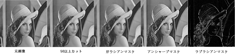
次の画像は、各処理をしたサンプル画像です。

周波数特性は、


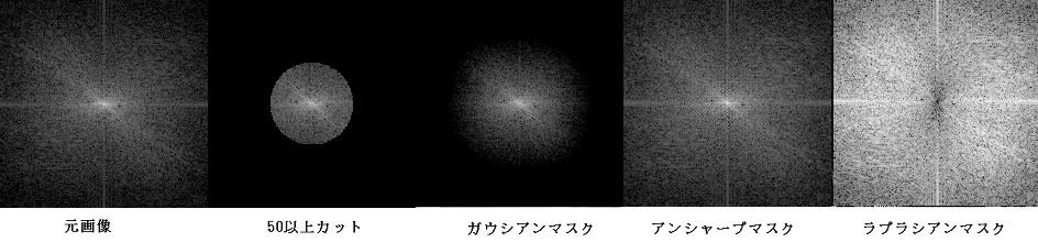
　単に５０以上をカットした場合は、画像に縞模様が発生します。
ガウシアンマスクを適用すると、通常のガウシアンマスクとなんら変わらない綺麗なボケ画像となります。
更に、ガウシアンマスクのボケ画像を利用して、アンシャープを行うと、通常のアンシャープと、そん色ない結果が得られました。
ラプラシアンマスクの場合、直流、低周波成分が少なくなり、高周波成分が多くなっています。
ラプラシアンマスクの場合、ピーク値がプラス側とマイナス側があるのですが、プラス側だけ表示しています。

　プログラムは、グレイ画像のみ作成しましたが、三色それぞれに同じ処理をすれば、カラーでの処理も可能です。

// ラプラシアン　アンシャープマスク
procedure TForm1.LaplacianBtnClick(Sender: TObject);
const
  // ラプラシアンマスク
  cvn = 3;
  conv : array[0..cvn - 1, 0..cvn - 1] of double = ((1,  1, 1),
                                                    (1, -8, 1),
                                                    (1,  1, 1));
  // ガウシアンマスク
  gaus = 5;
  Gaussian5X5 : array[0..4, 0..4] of double = ((1,  4,  6,  4, 1),
                                               (4, 16, 24, 16, 4),
                                               (6, 24, 36, 24, 6),
                                               (4, 16, 24, 16, 4),
                                               (1,  4,  6,  4, 1));
var
  conv_real : D2array;
  conv_image : D2array;
  half_cw : integer;
  half_ch : integer;
  nx, ny, x, y: integer;
  ar : D2array;            // データ実数部（入出力兼用)
  ai : D2array;            // データ虚数部（入出力兼用)
  r, i : Double;
  norm, max : Double;
  data : Double;
  Gauss : array[0..4, 0..4] of double;
  PBA : PByteArray;
  WP, DI : Integer;
  Total : Double;
begin
  LaplacianBtn.Enabled := False;
  OPT := 0;                // OPT = 0　通常のＤＦＴ（直流分が左端）
  if Checkbox1.Checked then OPT := 1;
  setlength(conv_real, GHeight, GWidth);
  setlength(conv_image, GHeight, GWidth);
  setlength(ar, GHeight, GWidth);
  setlength(ai, GHeight, GWidth);
  // ガウシアンマスクの設定
  if (RadioGroup1.ItemIndex = 1) or (RadioGroup1.ItemIndex = 2) then begin
    // Gaussianマスクの値変換 合計値が１になるように変換します
    total := 0;
    for y := 0 to 4 do
      for x := 0 to 4 do
        total := total + Gaussian5X5[y, x];
    for y := 0 to 4 do
      for x := 0 to 4 do
        Gauss[y, x] := Gaussian5X5[y, x] / total;
    // 拡張マスクの設定
    half_cw := gaus div 2;
    half_ch := gaus div 2;
    for y := 0 to gaus - 1 do
      for x := 0 to gaus -1 do begin
        nx := GWidth - half_cw + x;
        ny := Gheight - half_ch + y;
        if nx >= GWidth then nx := nx - GWidth;
        if ny >= Gheight then ny := ny - GHeight;
        conv_real[ny][nx] := Gauss[y][x];
      end;
  end;
  // ラプラシアンマスクの設定
  if RadioGroup1.ItemIndex = 0 then begin
    half_cw := cvn div 2;
    half_ch := cvn div 2;
    for y := 0 to cvn - 1 do
      for x := 0 to cvn -1 do begin
        nx := GWidth - half_cw + x;
        ny := Gheight - half_ch + y;
        if nx >= GWidth then nx := nx - GWidth;
        if ny >= Gheight then ny := ny - GHeight;
        conv_real[ny][nx] := conv[y][x];
      end;
  end;
  // 原画像を読み込み，２次元ＦＦＴの入力データに変換します
  for y := 0 to GHeight - 1 do
    for x := 0 to GWidth - 1 do begin
      ar[y, x] := GrayMat[y][x];
      ai[y, x] := 0.0;
    end;
  // 拡張したマスクをフーリエ変換します
  // 注　マスクの場合、変換時、データー数による除算処理をしないようにします
  if fft2(conv_real, conv_image, 2, Y_EXP, X_EXP) = -1 then begin
    exit;
  end;
  // ２次元ＦＦＴを実行し 原画像を周波数成分に変換します
  if fft2(ar, ai, 1, Y_EXP, X_EXP) = -1 then begin
    exit;
  end;
  // アンシャープネス
  if RadioGroup1.ItemIndex = 2 then begin
    for x := 0 to GWidth - 1 do
      for y := 0 to GHeight - 1 do begin
        // ボケ画像の生成
        r := ar[y][x] * conv_real[y][x] - ai[y][x] * conv_image[y][x];
        i := ar[y][x] * conv_image[y][x] + ai[y][x] * conv_real[y][x];
        // 差分計算
        r := ar[y][x] - r;
        i := ai[y][x] - i;
        // 元データーに差分加算
        ar[y][x] := ar[y][x] + r;
        ai[y][x] := ai[y][x] + i;
      end;
  end;
  // ガウシアン　ラプラシアン
  if (RadioGroup1.ItemIndex = 1) or (RadioGroup1.ItemIndex = 0) then begin
    for x := 0 to GWidth - 1 do
      for y := 0 to GHeight - 1 do begin
        // ボケ画像の生成
        ar[y][x] := ar[y][x] * conv_real[y][x] - ai[y][x] * conv_image[y][x];
        ai[y][x] := ar[y][x] * conv_image[y][x] + ai[y][x] * conv_real[y][x];
      end;
  end;
  // チェックボックスにチェックが有ったら周波数表示
  // 無い場合は、画像に逆変換表示
  if CheckBox1.Checked then begin
    // ＦＦＴ結果を画像化
    max := 0;
    for y := 0 to GHeight - 1 do
      for x := 0 to GWidth - 1 do begin
        norm := ar[y, x] * ar[y, x] + ai[y, x] * ai[y, x]; // 振幅成分計算 パワースペクトル
        if norm <> 0 then norm := ln(norm); // 表示の為対数変換
        ar[y, x] := norm;
        if norm > max then max := norm;     // 最大値検索
      end;
    for y := 0 to GHeight - 1 do
      for x := 0 to GWidth - 1 do
        ar[y, x] := ar[y, x] * 255 / max;    // 画像用に 最大値を 255に設定
  end
  else begin
    // 逆ＦＦＴを実行して，フィルタ処理された周波数成分を画像に戻します
    if fft2(ar, ai, -1, Y_EXP, X_EXP ) = -1 then begin
      exit;
    end;
  end;
  // 結果を画像データに変換
  for Y := 0 to Gheight - 1 do begin
    PBA := OutputBitmap.ScanLine[Y];
    for X := 0 to GWidth - 1 do begin
      data := ar[y, x];
      if data > 255 then data := 255;
      if data < 0 then data := 0;
      DI := Round(data);
      WP := X * 3;
      PBA[WP] := DI;
      PBA[WP + 1] := DI;
      PBA[WP + 2] := DI;
    end;
  end;
  Image1.Canvas.StretchDraw(VRect, OutputBitmap); // 出力枠に変倍出力
  LaplacianBtn.Enabled := True;
end;

　プログラムの全ての内容についてはダウンロードして下さい。
サンプルプログラムは、ＦＦＴを使用しているので、データー数が２の累乗個に限られます。
２の累乗個以外の場合は、フーリエ変換部に通常のＤＦＴを使用して下さい。

　　　　 　FFT2Laplacian.zip

画像処理一覧へ戻る

　　　　　　最初に戻る